Comparison of Optimizers in Neural Networks

Abstract

Recent state-of-art successes in deep learning have shown that neural network is a powerful model for various tasks. Since training a deep neural network is usually complex and time-consuming, many methods are applied to speed up this process. As for optimization in neural network, gradient based algorithm is used as the optimizer which coordinates the forward inference and backward gradients of network and reduces the loss. Different gradient algorithms differ at the convergence rate and final performance. This blog gives a survey and some analysis on these algorithms by making a comparison in different datasets with different network architectures.

Introduction

In machine learning applications, gradient based algorithms are popular for training neural networks. Recently, many improved algorithms based on Gradient Descent were presented to boost up the training process like Nesterov, Adagrad, Rmsprop, Adadelta and Adam. All of them are first-order optimization methods and they perform parameter updating during backpropagation to reduce loss of network.

In this work, we first introduce the different variants of Gradient Descent. Therefore, to illustrate the performance of each optimizer, several experiments are taken to evaluate the benchmark. In addition, we introduce several works that are related to optimization in neural network.

Overview of Optimizers

In this section, we first introduce the basic ideas for each optimizer. The updating rules are mainly based on this paper(ruder2016overview).

Overall, people are solving empirical risk minimization(ERM). Basically, for each sample $i$ , we define a loss $J_i(\theta)$ , the objective function is

$J(\theta) = \frac{1}{n}\sum_i^n J_i(\theta)$

To find a best solution $\theta$ , which minimizes the objective function, Gradient Descent is applied, as shown in Algorithm Batch Gradient Descent. It will update parameters in the opposite direction of the gradient of objective function. Learning rate $\eta$ is the step size we take to perform weight updating.

Algorithm Batch Gradient Descent

$\theta_t \gets \theta_{t-1} - \eta \frac{1}{n}\sum_i^n \triangledown J_i(\theta)$ .

Assume $x^*$ is the best solution, we could get

$f(x_t) - f(x^*) \leq \frac{\lVert x_0 - x^* \rVert ^2}{2\eta t}$

As we know, the convergence rate of gradient descent is $O(\frac{1}{t})$ . In addition, we also know that for a L-smooth function( $L$ is the Lipchitz parameter), to make sure the Gradient Descent will converge, we should pick a learning rate $\eta$ smaller than $\frac{1}{L}$ .

When it comes to large-scale dataset, the training samples can be millions. Gradient Descent will calculate gradients over whole dataset to perform one iteration. It is impossible to keep every gradient in memory. It is also wasteful when there are some redundant samples in dataset. By carefully choosing the learning rate, Gradient Descent is sure to converge into a global minima in convex optimization and a local minima for non-convex optimization.

Online learning(Algorithm Online Learning) is an extreme case that we update parameters for each point. As the training point could be random, there is fluctuation in train process. However, the fluctuation also makes the algorithm possible to jump out a local minima into a better one. But sometimes, the online learning may not converge.

Algorithm Online Learning

$\theta_t \gets \theta_{t-1} - \eta \triangledown J_i(\theta; X_i, Y_i)$ .

def gd(x_start, step, gradient, iteration=50):
    x = np.array(x_start, dtype='float64')
    passing_dot = [x.copy()]
    for _ in range(iteration):
        grad = gradient(x)
        x -= grad * step
        passing_dot.append(x.copy())
        if abs(sum(grad)) < 1e-6:
            break;
    return x, passing_dot

Mini-batch gradient descent(Algorithm SGD) is the most popular algorithm in neural networks, which takes the advantages of Online Learning and Batch Gradient Descent. Mini-batch gradient descent updates parameters for every small batch in training samples. Compared to Online Learning, it could reduce the variance during training. It is also able to jump out a local minima. Generally, when people say Stochastic Gradient Descent (SGD) in neural networks, it stands for mini-batch gradient descent.

Algorithm SGD
$\theta_t \gets \theta_{t-1} - \eta \triangledown J_i(\theta; X_{i:i+n}, Y_{i:i+n})$

SGD will be greatly affected by some large gradients in some dimensions. It has trouble in areas where the surface curves is much more steeply in one dimension than others. Hence it is hard for SGD to jump out saddle point.

Momentum(qian1999momentum)(Algorithm Momemtum) is used to boost the speed when the gradient is small in some directions. For each iteration, it will combine the direction of gradient and its last position vector, which may accelerate SGD in the relevant direction. $\gamma$ is the parameter stands for the factor of last positionvector. Momentum increases the updating speed in the same directions and reduces speed when the gradients change directions. It is like a “heavy ball”, during updating, inertia makes it moves faster in its direction. By accumulating speed in gradient, SGD with Momentum could overcome the defect of original SGD.

Algorithn Momentum

$v_t \gets \gamma v_{t-1} + \eta \nabla_\theta J( \theta)$ .

$\theta \gets \theta - v_t$ .

def momentum(x_start, step, g, discount=0.7, iteration=50):
    x = np.array(x_start, dtype='float64')
    passing_dot = [x.copy()]
    pre_grad = np.zeros_like(x)
    for _ in range(iteration):
        grad = g(x)
        pre_grad = pre_grad * discount + grad
        x -= pre_grad * step
        passing_dot.append(x.copy())
        if abs(sum(grad)) < 1e-6:
            break;
    return x, passing_dot

However, in some cases, if the momentum parameter (\gamma) is too large, this algorithm may go across the minima. Back to ball example, it is like when the ball reaches a minima, due to the effect of inertia(momentum), the ball keeps going and makes loss function increase.

Therefore, Nesterov Accelerated Gradient(Algorithm NAG) is introduced to fix this disadvantage.

Algorithm NAG

$v_t \gets \gamma v_{t-1} + \eta \nabla_\theta J( \theta - \gamma v_{t-1} )$ .

$\theta \gets \theta - v_t$ .

def nesterov(x_start, step, gradient, discount=0.7, iteration=50):
    x = np.array(x_start, dtype='float64')
    passing_dot = [x.copy()]
    pre_grad = np.zeros_like(x)
    for _ in range(iteration):
        x_future = x - step * discount * pre_grad
        grad = gradient(x_future)
        pre_grad = pre_grad * 0.7 + grad 
        x -= pre_grad * step
        passing_dot.append(x.copy())
        if abs(sum(grad)) < 1e-6:
            break;
    return x, passing_dot

NAG is like a prediction, it will first consider the momentum direction, calculate the gradient on that position, then it combines these two directions to make an update. The comparison of strategies between Momentum and NAG is shown in Figure 1.

momentum_nag

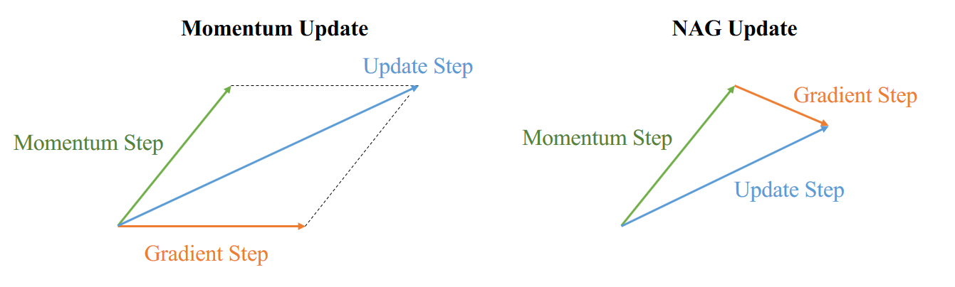
Figure 1. Comparison of strategy between Momentum and NAG. Momentum(left) first computes the current gradient (orange vector) and then takes a big jump in the direction of the updated accumulated gradient (green vector). NAG(right) first makes a big jump in the direction of the previous accumulated gradient (green vector). As follows, NAG measures the gradient and then makes a correction (orange vector).

This strategy of NAG prevents the ball from going too fast and makes the ball stop before gradient increases. This property results in increased responsiveness, which has significantly increased the performance of RNN.

So far, these two improvements are based on momentum. However, all of them use a same learning rate for all parameters, when there are is some noise in one dimension, it may influence all parameters. As a result, it is hard to find a suitable learning rate when we have a high-dimensional dataset. Therefore, there are some works on tuning learning rate individually.

Adagrad(duchi2011adaptive)(Algorithm Adagrad) is one of them. It adapts the learning rate w.r.t. each parameter based on previous gradients( $G_t = \sum_{i=1}^{t} g_{i}^2$ ). Here $G_t$ is a diagonal matrix where each diagonal element is the sum of the squares of the gradients w.r.t. $\theta$ up to time step. This is then used to normalize the parameter update step. $\epsilon$ is a very small number set to prevent the division by zero. Adagrad keeps track of gradient updating and performs larger updates for infrequent parameters, whereas smaller updates for frequent parameters. This means Adagrad is more suitable for sparse data.As normalization is performed during training, we do not need to manually tune the learning rate. People may set a default learning rate as 0.01.

Algorithm Adagrad

$g_{t} \gets \nabla_\theta J( \theta_{t-1} )$ .

$G_{t} \gets G_{t} + g_t \odot g_t$ .

$\theta_{t} \gets \theta_{t-1} - \dfrac{\eta}{\sqrt{G_{t} + \epsilon}} \odot g_{t}$ .

def adagrad(x_start, step, gradient, delta=1e-8, iteration=50):
    x = np.array(x_start, dtype='float64')
    passing_dot = [x.copy()]
    sum_grad = np.zeros_like(x)
    for _ in range(iteration):
        grad = gradient(x)
        sum_grad += grad * grad
        x -= step * grad / (np.sqrt(sum_grad) + delta)
        passing_dot.append(x.copy())
        if abs(sum(grad)) < 1e-6:
            break;
    return x, passing_dot

One weakness of Adagrad is that, due to the accumulation of squared gradients in denominator, learning rate may shrink and eventually converge to zero. To overcome this defect, Adadelta(zeiler2012adadelta)(Algorithm Adadelta) is derived from Adagrad.

Algorithm Adadelta

$g_{t} \gets \nabla_\theta J( \theta_{t-1} )$ .

$G_{t} \gets \gamma G_{t} + (1-\gamma)g_t \odot g_t$ .

$\Delta \theta_t \gets -\frac{\sqrt[]{\Delta_{t-1}+\epsilon}}{\sqrt{G_{t} + \epsilon}} \odot g_{t}$ .

$\theta_t \gets \theta_{t-1} + \Delta \theta_t$ .

$\Delta_t \gets \gamma \Delta_{t-1} + (1-\gamma)\Delta \theta_t \odot \Delta \theta_t$ .

def adadelta(x_start, step, gradient, momentum=0.9, delta=1e-1, iteration=50):
    x = np.array(x_start, dtype='float64')
    sum_grad = np.zeros_like(x)
    sum_diff = np.zeros_like(x)
    passing_dot = [x.copy()]
    for _ in range(iteration):
        grad = gradient(x)
        sum_grad = momentum * sum_grad + (1 - momentum) * grad * grad
        diff = np.sqrt((sum_diff + delta) / (sum_grad + delta)) * grad
        x -= step * diff
        sum_diff = momentum * sum_diff + (1 - momentum) * (diff * diff)
        passing_dot.append(x.copy())
        if abs(sum(grad)) < 1e-6:
            break;
    return x, passing_dot

Adadelta aims at improving the shrinkage of learning rate. Instead of accumulating all past squared gradients, Adadelta restricts the window of accumulated past gradients to some fixed size. It is a decaying average of all past squared gradients, like an invert momentum in learning rate. As we can see from the update rule, we do not need to set a default learning rate for Adadelta.

RMSprop(hinton2012lecture)(Algorithm Rmsprop) was developed independently around the same time of Adadelta to resolve diminishing learning rates in Adagrad. The idea is same as Adadelta. By keeping a decaying squared gradients, RMSprop will not get monotonically smaller. Therefore, people may set a very small value for default learning rate, like 0.001. In addition, people often set the $\gamma$ to 0.9.

Algorithm Rmsprop

$g_{t} \gets \nabla_\theta J( \theta_{t-1} )$ .

$G_{t} \gets \gamma G_{t} + (1-\gamma)g_t \odot g_t$ .

$\theta_{t} \gets \theta_{t-1} - \dfrac{\eta}{\sqrt{G_{t} + \epsilon}} \odot g_{t}$ .

def rmsprop(x_start, step, gradient, rms_decay=0.9, delta=1e-8, iteration=50):
    x = np.array(x_start, dtype='float64')
    sum_grad = np.zeros_like(x)
    passing_dot = [x.copy()]
    for _ in range(iteration):
        grad = gradient(x)
        sum_grad = rms_decay * sum_grad + (1 - rms_decay) * grad * grad
        x -= step * grad / (np.sqrt(sum_grad) + delta)
        passing_dot.append(x.copy())        
        if abs(sum(grad)) < 1e-6:
            break;
    return x, passing_dot

If we combine the momentum and individual learning rate, we get Adam(kingma2014adam)(Algorithm Adam), which stands for adaptive moment estimation. In addition to storing an exponentially decaying average of past squared gradients like Adadelta and RMSprop, Adam also keeps an exponentially decaying average of past gradients, similar to momentum.

Algorithm Adam

$g_{t} \gets \nabla_\theta J( \theta_{t-1} )$ .

$m_t \gets \beta_1 m_{t-1} + (1-\beta_1)g_t$ .

$v_t = \beta_2 v_{t-1} + (1 - \beta_2) g_t^2$ .

$\hat{m}_t = \dfrac{m_t}{1 - \beta^t_1}$ .

$\hat{v}_t = \dfrac{v_t}{1 - \beta^t_2}$ .

$\theta_{t} = \theta_{t-1} - \dfrac{\eta}{\sqrt{\hat{v}_t} + \epsilon} \hat{m}_t$ .

def adam(x_start, step, gradient, beta1=0.9, beta2=0.999, delta=1e-8, iteration=50):
    x = np.array(x_start, dtype='float64')
    sum_m = np.zeros_like(x)
    sum_v = np.zeros_like(x)
    passing_dot = [x.copy()]
    for _ in range(iteration):
        grad = gradient(x)
        sum_m = beta1 * sum_m + (1 - beta1) * grad
        sum_v = beta2 * sum_v + (1 - beta2) * grad * grad
        correction = np.sqrt(1 - beta2 ** i) / (1 - beta1 ** i)
        x -= step * sum_m / (np.sqrt(sum_v + delta))
        passing_dot.append(x.copy())
        if abs(sum(grad)) < 1e-6:
            break;
    return x, passing_dot

By adjusting first and second moment, Adam utilizes initialization bias correction terms. The method combines the advantages of two recently popular optimization methods: the ability of AdaGrad to deal with sparse gradients, and the ability of RMSProp to deal with non-stationary objectives. Author in the paper suggests that good default settings for parameter are $\eta=0.001, \beta_1=0.9, \beta_2=0.999, \epsilon=10^{-8}$ .

Experiment Results

To test these algorithms, we compared the performance of 7 optimizers on several benchmarks: simple convex function, saddle point case, MNIST and CIFAR-10.

Simple Convex Function

This simple convex case is designed to illustrate basic idea about these optimization algorithms. Here, we set a toy convex function as

$f(x, y)=x^2 + 10y^2$

xi = np.linspace(-8, 8, 1000)
yi = np.linspace(-8, 8, 1000)
X,Y = np.meshgrid(xi, yi)
Z = X * X + 10 * Y * Y

def contour(X,Y,Z, arr = None):
    plt.figure(figsize=(10, 10))
    xx = X.flatten()
    yy = Y.flatten()
    zz = Z.flatten()
    plt.contourf(X, Y, Z, 20, cmap=plt.get_cmap('viridis'))
    if arr is not None:
        arr = np.array(arr)
        for i in range(len(arr) - 1):
            plt.xlim(-8, 8)
            plt.ylim(-8, 8)
            plt.plot(arr[i:i+2,0],arr[i:i+2,1], color='white')
        
contour(X,Y,Z)

The global minima is obtained at $(0, 0)$ . To begin with the training process, we set the start point at $(7, 5)$ .

We first test the performance of original SGD method. From the result shown in Figure 2, for targeted problem, it is important to choose a suitable learning rate. Small default learning rate may lead to a very slow training process and “under-fit”. Meanwhile, larger learning rate may give us a faster converge rate, as well as risks in diverging. Generally, we should avoid setting too large learning rate and introduce a decaying rate in step size in real application.

sgd

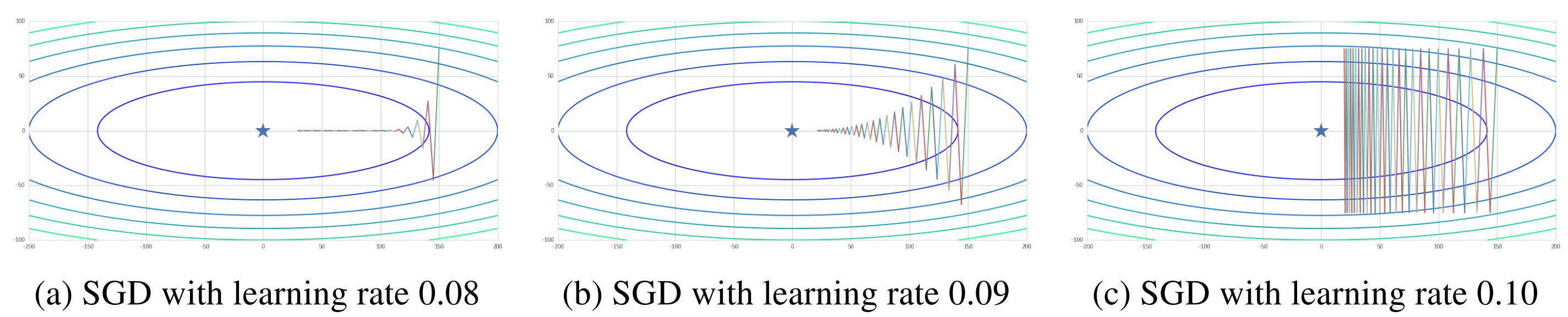
Figure 2. SGD with different learning rates

Figure 3 illustrates the influence of momentum factor $\gamma$ . Large momentum could greatly boost up the training process, but also bring more fluctuation during training. However, by applying NAG, we could smooth the updating process and prevent loss value from fluctuating around minima.

Momentum

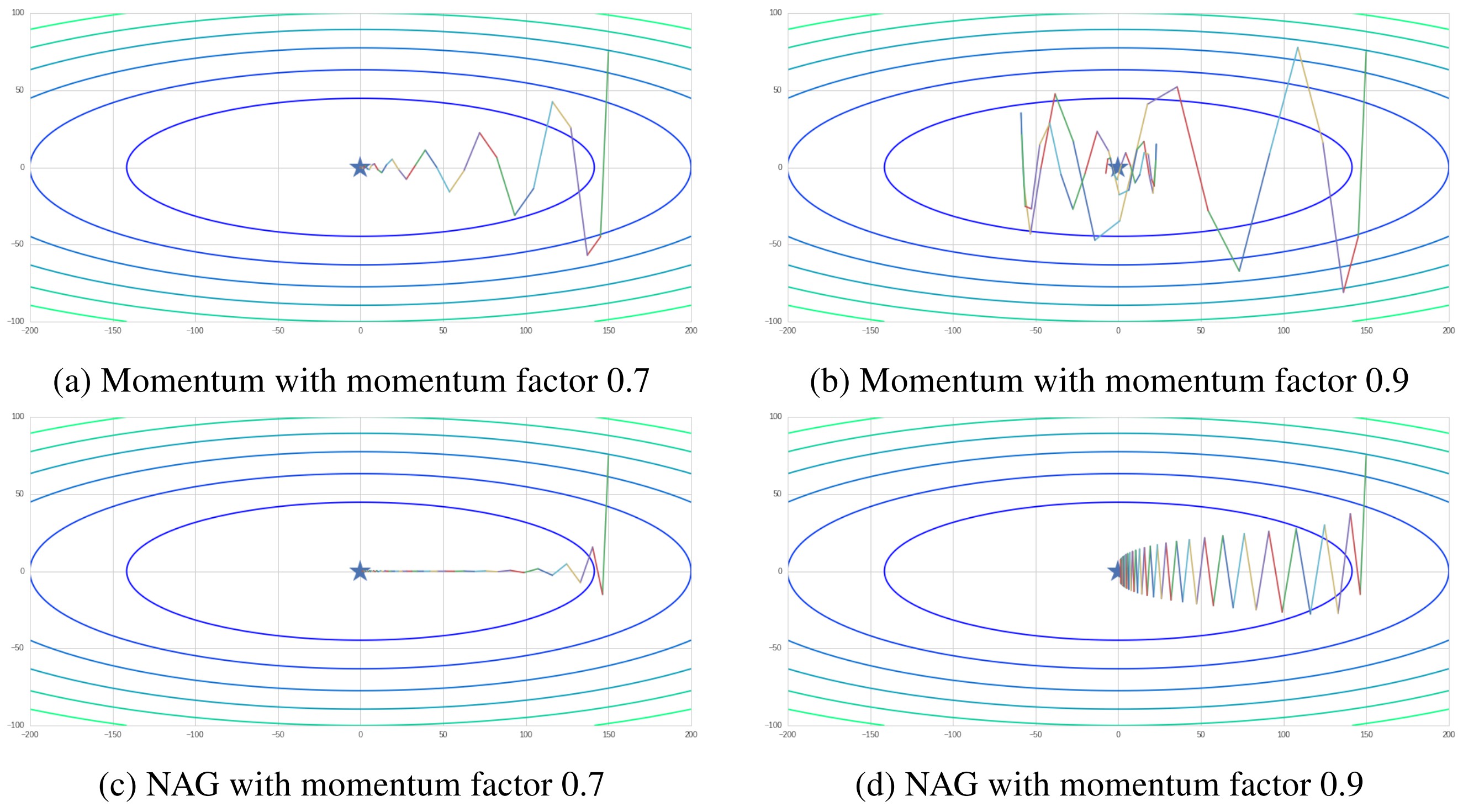
Figure 3. Momentum and NAG with different gamma values

Adaptive learning rate methods (Adagrad, Adadelta, RMSprop and Adam) could reduce the influence of anomalous gradients in some dimensions. From the Figure 4, we could find that all of these methods take very smooth updates. Due to the normalization of learning rate, we set a larger learning rate to these methods. Compared to momentum based methods, they move toward minima at the beginning of training. Specially, as Adam applies momentum and adaptive learning rate, its movement trace is like a circle around minima. It achieves global minima faster than others even with a halved learning rate.

adaptive

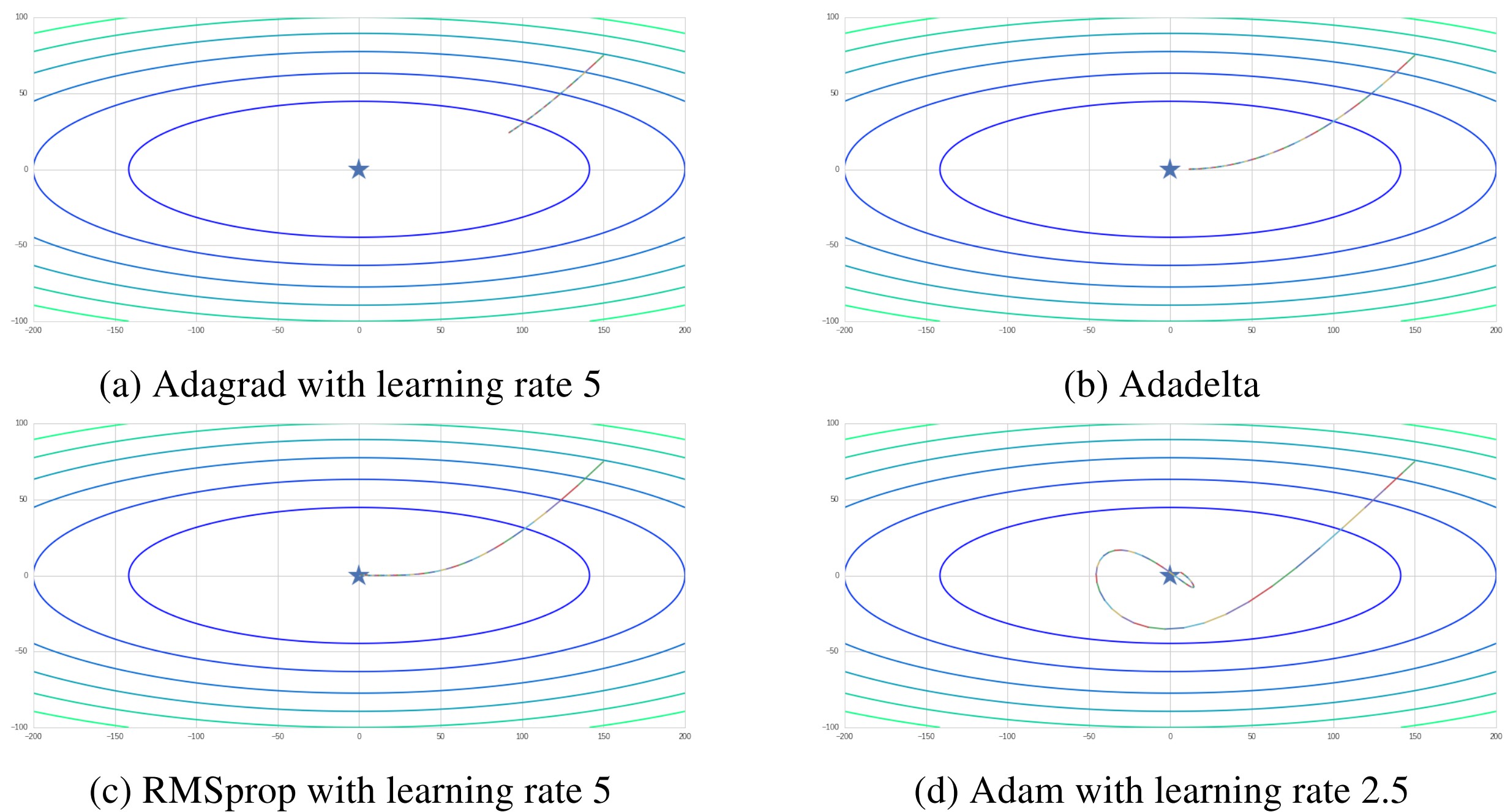
Figure 4. Comparison between adaptive learning rate methods

Saddle Point

For a long time in history, it has been universally accepted that the difficulty of training neural networks comes from too much local minimas in loss surface. As a result, optimizer is likely to get stuck in some of them and get a poor performance.

However, a paper by Dauphin, Yann N., et al(dauphin2014identifying) suggests that, based on results from statistical physics, random matrix theory, neural network theory and empirical evidence, this difficulty originates from the proliferation of saddle points instead of local minima, especially in high dimensional problems. Such saddle points are surrounded by high error plateaus that can dramatically slow down learning.

Since current optimizers are all based on gradient, when they come to saddle point, where some gradients are 0 and the Hessian is indefinite, updating process could be very slow. Here we set a classic saddle point case $f(x, y) = x^2 - y^2$ to evaluate these algorithms. The saddle point case is shown in Figure 5. $(0, 0)$ is the saddle point where the gradients of x, y are zero and the Hessians are not all positive.

saddle

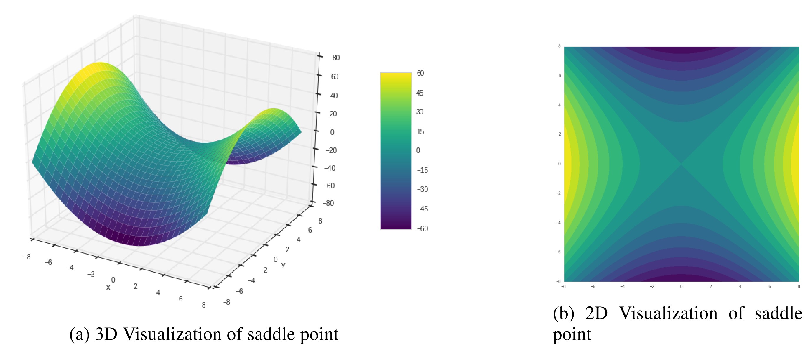
Figure 5. Visualization of a simple saddle point case

To test the performance of all optimizers, we select a start point at $(7, 0.001)$ , where the gradient in y is nearly zero.

As shown in Figure 6, original SGD has trouble getting out saddle point, if we set a decay in learning rate, SGD may get stuck in $(0, 0)$ . Similar to previous test, Momentum could boost up the training speed, but may also make some redundant updates. NAG works well in navigating ravines, where some gradients are much more steeply than in others.

saddle

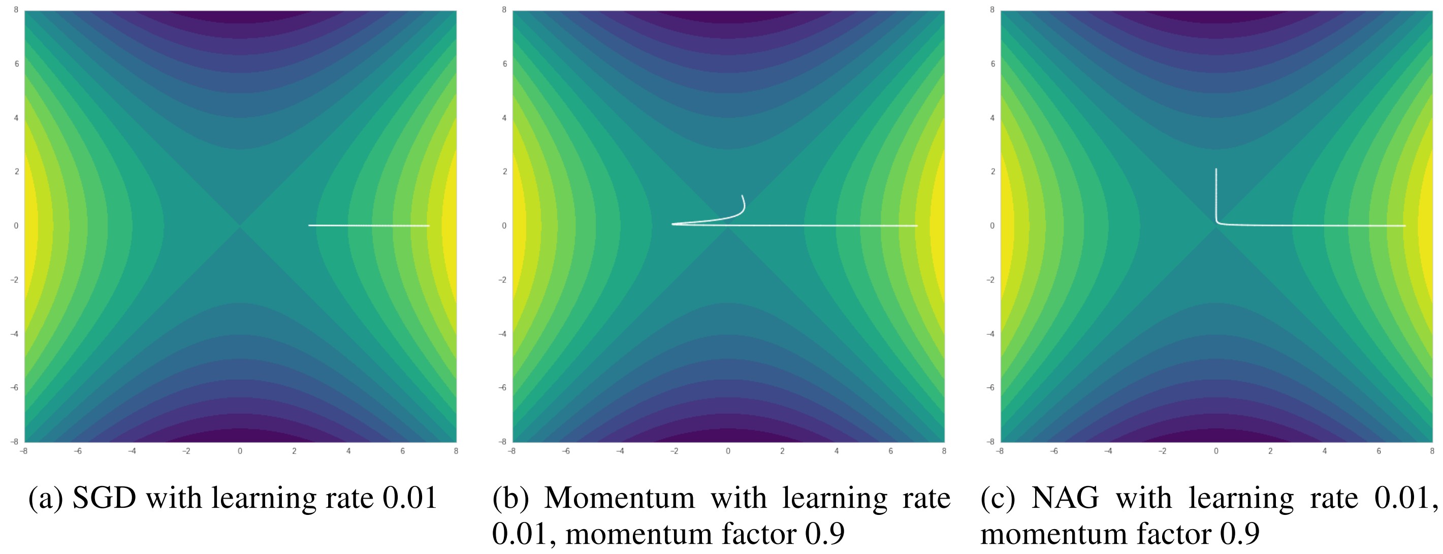
Figure 6. Momentum with learning rate 0.01, momentum factor 0.9

Adaptive learning methods are designed to solve sparse gradient. By accumulating history gradients and normalizing learning rate for each dimension, they are much less likely to get struck at saddle point. However, if $(0, 0)$ happens to be a global minima(not in this saddle case), these algorithms may miss it. Generally, Adam is still the best one that escapes saddle point with fewest iterations and fastest rate.

adaptive

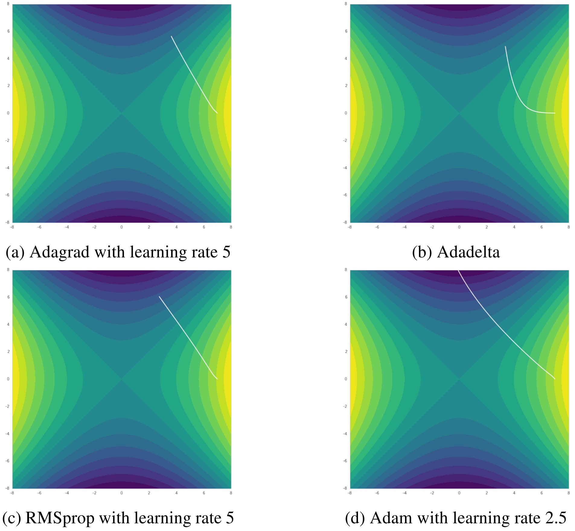
Figure 7. Comparison between adaptive learning rate methods in saddle point case

MNIST

MNIST is a classic and popular benchmark to test algorithms in computer vision. It is a database of handwritten digits and the goal is to classify images into correct label. We test these 7 algorithms by Logistic Regression, Multi-layer Perceptron and Convolutional Neural Network on it.

Logistic Regression

Logistic Regression is a popular linear classifier. The model can be written as

$P(Y=i | x, W, b) = softmax_i(Wx+b) = \frac{e^{W_ix+b_i}}{\sum_j e^{W_jx+b_j}}$

We set the loss function as the negative log-likelihood function. The likelihood function $L$ and loss $l$ are defined as:

$L(W,b) = \sum log(P(Y=y^{(i)}|x^{(i)}, W, b))$ $l(W,b) = -L(W,b) = -\sum log(P(Y=y^{(i)}|x^{(i)}, W, b))$

The result is presented in Figure 8. All algorithms converge with a similar rate. As Logistic Regression is a convex problem, all optimizers finally converge to a same solution after many iterations(too long to show on figure).

mnist_log

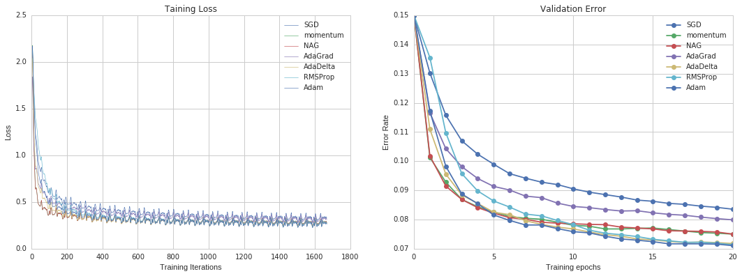
Figure 8. Results for Logistic Regression in MNIST

Multi-layer Perceptron

Multi-layer Perceptron (MLP) is a kind of supervised learning algorithm. It contains multiply hidden layers which is the prototype of deep learning.Since backpropagation algorithm was invented in 1980s, people have been using it to train neural networks. With the support of multiply hidden layers, it can handle non-linear classification and it is able to learn online with partial fit. However, the loss function of MLP is non-convex, different random states can lead to different validation accuracy. In this test, we set up a MLP with 2 hidden layers and 500 nodes in each hidden layer.

From Figure 9, Adam performs best out of all optimizers. In fact, Adam works pretty well on relatively large datasets (with thousands of training samples or more) in terms of both training time and validation score. In Python package Scikit-Learn, it is recommended as the default solver. Specially, For small datasets, a quasi-Newton method, like Limited-memory BFGS, can converge faster and perform better.

mnist_mlp

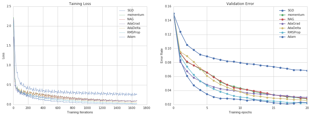
Figure 9. Results for Multi-layer Perceptron in MNIST

CNN

CNN is a special kind of multi-layer neural networks. Recently, CNN has achieved many state-of-art results in computer vision.

In this test, we apply LeNet-5 as the training model. It contains 7 layers: $Input->Conv2D->Pool->Conv2D->Pool->FC->FC->Output$

The loss function is Cross Entropy Loss. In order to get a reliable conclusion, different initial weights are tested to obtain a averaged result.

By the result in Figure 10, all optimizers show a similar converge rate. In addition, except original SGD and Adadelta, these optimizers are resemble both in final accuracy and loss.

mnist_cnn

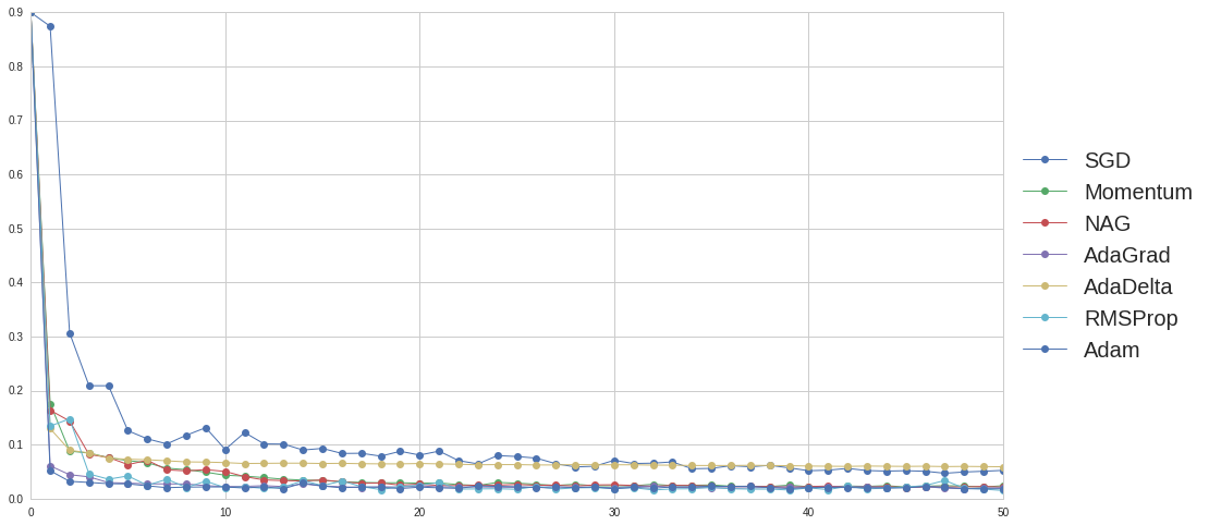
Figure 10. Results for Convolutional Neural Network in MNIST

CIFAR-10

Compared to other problems in computer vision, MNIST with binary value in only one channel is relatively simple. For applications in real scenes, the input could be images in RGB channels with higher resolution. To further investigate the performance of optimizers, we test them in CIFAR-10 dataset with Deep Residual Network.

Deep Residual Network by Kaiming He et al achieved state-of-art result in ImageNet 2015. The novel design of residual block makes it possible to train a deeper network. Due to the limitation on computing resource, we only tested ResNet with 18 layers. The result is presented in Figure 11.

cifar_cnn

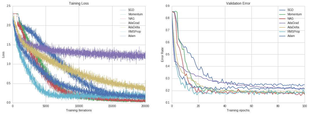
Figure 11. Results for Deep Residual Network in MNIST

One interesting observation is that, although SGD with momentum and NAG are not best in previous tests, additionally, they do not converge with a fastest rate, they achieve best accuracy when optimization converges. It could be a supporting evidence that illustrates why some researchers nowadays still prefer SGD with momentum.

More About Optimization

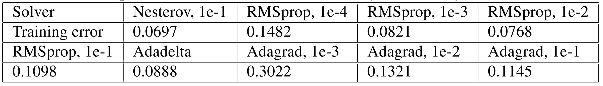
Since we haven’t tested in very large dataset with very complex network, we here cite some works by others. Facebook(gross2016training) has tested NAG, RMSprop, Adadelta and Adagrad with 110-layer Deep Residual Network on CIFAR-10.This result also supports that SGD with momentum is still the best solver for some problems, even in a very complex network. The author illustrates that “Alternate update rules may converge faster, at least initially, but they do not outperform well-tuned SGD in the long run.”

Table 1. Experiments on CIFAR-10 with 110-layer ResNet by Facebook

cifar_table

Visualization of loss surface

Usually, it could be hard to visualize loss surface for neural network of high dimension and non-convex optimization. One possible way is projecting the loss surface onto lower dimensions.

This is an interesting work related to a visualization of loss surface in Neural Networks by Daniel Jiwoong Im et al(im2016empirical). Through several experiments that are visualized on polygons, the authors try to show how and when these stochastic optimization methods find local minima.

visual

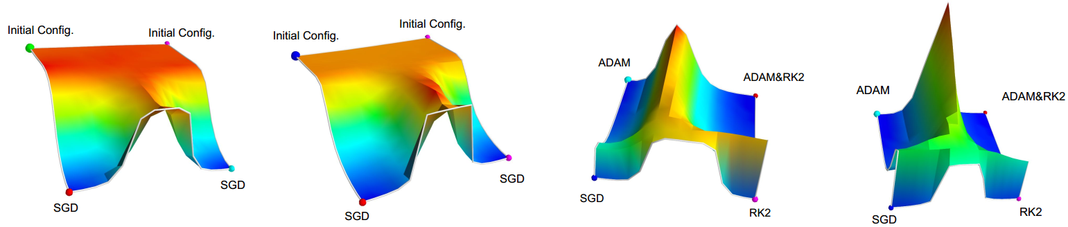
Figure 12. Left two: weights interpolated between two initial configurations and the final weight vectors learned using SGD. Right two: weights interpolated between the weights learned by four different algorithms.

Batch Normalization by Google(ioffe2015batch) is a recent method that greatly improves training speed. It has also been tested to be beneficial to final accuracy. Figure13 is an illustration on how BN affects the training process. From this figure, we may find that BN greatly reduces the plateau of loss function and makes updating easier for optimizer.

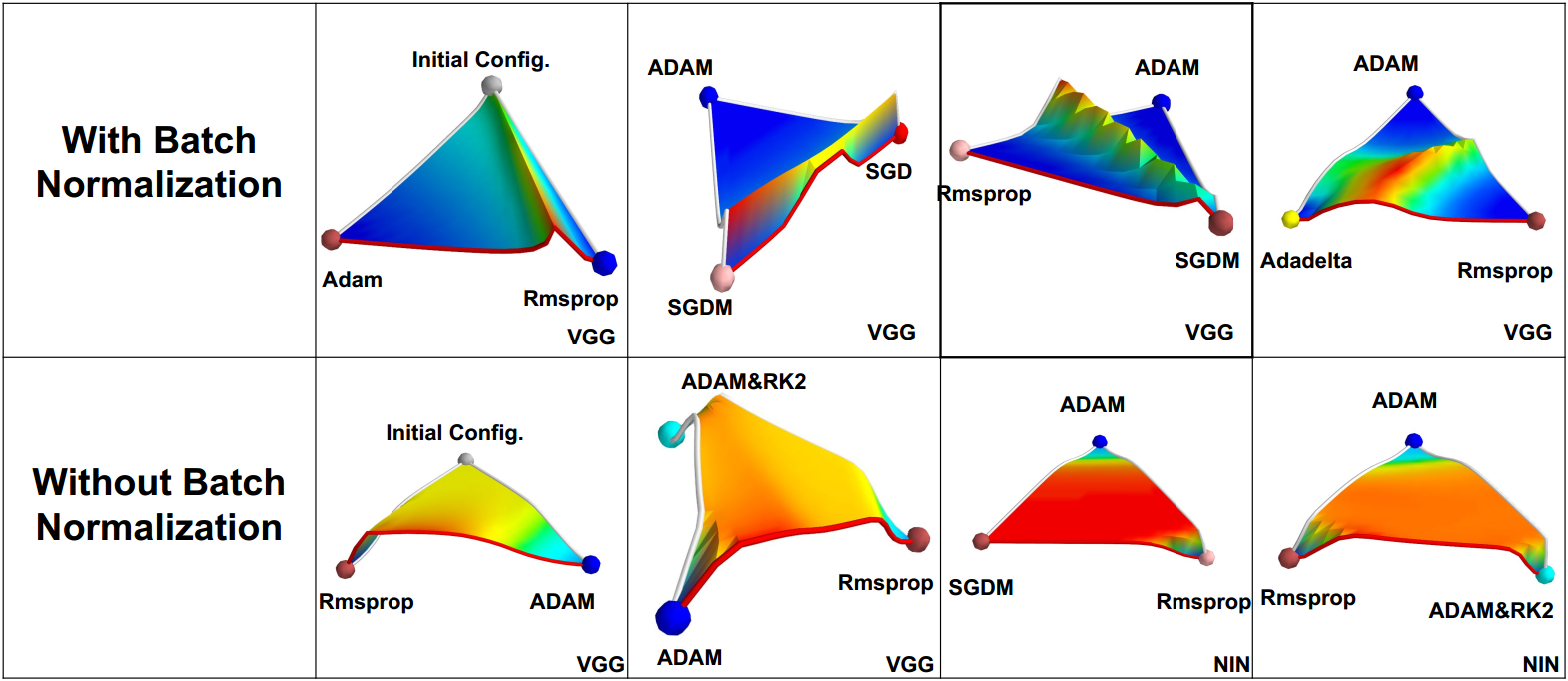
Figure 13. Visualization of the Loss Surface with and without batch-normalization by Daniel Jiwoong Im et al

Comparison between Gradient Descent and Newton’s methods

All optimizers mentioned in this report are kinds of first-order method. As for second-order method like Newton’s method, we need to maintain a complete approximated Hessian matrix or its inverse, which is not practical in large-scale optimization problem. Although people may use L-BFGS or stochastic L-BFGS in some neural networks and obtain a faster converging speed than first-order method, it only shows its advantage when it is close enough to minima. What’s more, as for L-BFGS, when we approximate Hessian by gradients in mini-batch, we introduce noise in computation, which may bring huge influence in calculus.

In most machine learning applications, people require less on the precision of exact minima i.e. it is acceptable when we get a relatively close approximation. In this case, it may cost more in extra computation for L-BFGS compared to performing more iterations in SGD. In addition, as we only need to tune learning rate in SGD, with a carefully selected learning rate,the optimization of Gradient Descent is promising to converge. As for L-BFGS, it may not converge in some non-convex cases.

Learning to learn by gradient descent by gradient descent

This is a recent interesting paper by Google DeepMind(andrychowicz2016learning). Instead of using a optimizer for general case, these authors came up with a new idea: use Recurrent Neural Network to tune the learning rate for gradient descent.

As discussed in this report, gradient based optimizer follows this general rule:

$\theta_t \gets \theta_{t-1}-\eta \triangledown f(\theta_{t-1})$

It is a reasonable inspiration that LSTM could be used to model the optimizer. Therefore, the network takes gradient as input and makes a prediction about the updating values. In other words, we could use LSTM to learn $\eta \triangledown f(\theta_{t-1})$ .

The training process can be described as follows. As for a target loss function $f(\theta)$ , we first randomly collect some $W$ and $y$ as training data. Based on $\theta$ in one moment $t$ , we calculate the value of $f$ and error $\triangledown_t$ w.r.t. $\theta$ .Next, we take $\triangledown_t$ and previous state of LSTM as input to get gradient. Finally, we update $\theta$ by gradient and use the loss to update parameters in LSTM.

In that paper, they show a very promising result in MNIST with MLP and CIFAR-10. Personally speaking, we think it could be the next breakthrough of optimization in Neural Networks.

Conclusion

In this blog, we introduce most popular algorithms in optimization inneural networks. Momentum and NAG are trying to improve original SGD by introducing suitablemomentum. In a different way, Adagrad, Adadelta, RMSprop are methods derived from SGD with adaptive learning rate. Finally, Adam combines these two strategies and is the theoretically best one. According to our results, Adam does work well in most cases. However, we also found that SGD with momentum is still the best choice considering robustness and final accuracy in some particular cases. As there are fewer tuning parameters in SGD, researchers could keep focus on model. With manually selected learning rate, SGD is guaranteed to converge to a local minima. Considering applications in real scenes, that is a very important property. Recently, a work by Google shows the possibility of training a optimizer forneural network by a neural network. This method is potential to be the next prevailing optimizer and enables neural networks to bootstrap. However, this novel method needs lots ofcomputation. From some implementations by others, we still can not reproduce the result of this method. Currently, there are still many problems to discover about optimization in neural networks.

Ruifan Yu

Welcome! My name is Ruifan Yu. I am currenly a Software Engineer in Google, exploring the fabulous ocean of Computer Science.