Abstract

Linear programming and feasibility problem are basic problems in convex optimization. So far, many algorithms have been developed to solve them. In this study-type project, we write a survey about a typical class of algorithms called cutting-plane method. The difference between cutting-plane methods lies in the way to select cutting point. We construct this report from the original cutting-plane method to the recent state-of-the-art method with an analysis on the running time and some proofs.

Introduction

In this blog, some cutting-plane methods are introduced. Generally, they are an important class of algorithm for analyzing feasible problem and linear problem. According to the way how the point is selected to feed oracle, there are cutting-plane methods using the center of gravity, the analytic center, the ellipsoid center, and the volumetric center, resulting in the difference on the number of separation oracle calls and the computing complexity for querying point. Among these methods, the optimal number for calling separation oracle is $O(n)$(the center of gravity), and the optimal method for computing querying point is $O(n^2)$(Lee, Sidford, Wong). In total running time, the best result so far is $O(n^3\log n)$.

Feasibility Problem

Definition(feasibility problem) : A feasibility problem is defined as

$$find ~ x$$ $$subject ~ to ~ f_i(x) \leq 0, \forall i$$

where in each constraint, $f_i$ is convex function.

The goal is to find a feasible solution $x$ that can satisfy all the constraints. For linear programming, we have linear constraints, note as $AX \leq B$ or $a_i^T x_i \leq b_i, \forall i$.

From Feasibility Problem to Optimization Problem

Definition(convex optimization problem) : A convex optimization problem is

$$\min f(x)$$ $$subject ~ to ~ g_i(x) \leq 0, \forall i$$

As for convex optimization problem, the set given by constraints should be a convex set. Let this set named $C$, and $x^*$ is the point in $C$ that minimizes $f(x)$, we assume that $x^*$ is contained in a ball with a small radius. The output of algorithms should be a point $x_T$ such that $x_T \in C$, and $f(x_T) - f(x^*) \leq \gamma$.

We can use the algorithm for feasibility problem in optimization problem with some modifications. From the algorithm, we obtain a feasible point $z$. Instead of returning the solution, we compute a vector $w$ such that $\{x: f(x) \leq f(z)\} \subseteq \{x:w^Tx \geq w^Tz\}$ and replace the vector returned by the oracle with it. Once $w$ is available, the remaining parts are the same as those in the feasibility problem. During iterations, we keep a track of $z_T$ and record the best point $z^*$. When the algorithm halts, we return $z^*$ as $x^*$.

Cutting Plane Method

Cutting-plane method is a class of methods for solving linear programming or feasibility problem. The basic idea is using a hyperplane to separate the current point from the optimal solution. According to this note(boyd2011localization), cutting-plane methods have these advantages:

• Cutting-plane methods supports black-box property, in other words, these methods do not need the differentiability of the objective and constraint functions. In each iteration, we can use subgradient as the approximation of gradient.
• Cutting-plane methods which can exploit certain structure can be faster than a general purpose interior-point method.
• Cutting-plane methods do not need to perform evaluation of the objective and constraint functions in each iteration. Which contrasts to interior-point method that requires evaluating both objective and constraint functions.
• Cutting-plane methods is well suitable for scalability. They can be used in complex problems with a very large number of constraints by decomposing problems into smaller ones that can be solved in parallel.

Separation Oracle

The basic assumption for cutting-plane method is the existence of Separation Oracle for given sets or functions.

Definition(Hyperplane) : A Hyperplane is the set of points satisfying the linear equation $ax=b$, where $a,b,x \in R^n$

Lemma : if $K \subseteq R^n$ is a convex set and $p \in R^n$ is a given point, then one of the two condition holds

1. $p \in K$.
2. there is a hyperplane that separates $p$ from $K$.

Definition(Separation Oracle for a set) : Given a set $K \subseteq R^n$ and $\delta \geq 0$, a $\delta$-separation oracle for $K$ is a function such that for an input $x \in R^n$, it either outputs “successful” or a halfspace $H=\{z: c^Tz \leq c^Tx+b\} \supseteq K$ with $b \leq \delta \lVert c \rVert _2$ and $c \neq 0$.

Definition(Separation Oracle for a function) : For a convex function $f$, let $\eta \geq 0$ and $\delta \geq 0$, a $(\eta, \delta)$-separation oracle for $f$ is a function such that for an input $x \in dom(f)$, it either tell if

$$f(x) \leq \min_{y \in dom(f)}{f(y) + \eta}$$

or outputs a halfspace $H$ such that

$\{z: f(z) \leq f(x)\} \subset H := \{z: c^T z \leq c^T x +b\}$, with $b \leq \delta \lVert c \rVert$ and $c \neq 0$.

Generally, we set $\delta=0$, and note $SO(K)$ as the running time complexity of this oracle.

Cutting-Planes

To conclude, the feasibility problem can be described as to find a point in a convex set or assert that there is no feasible point in this convex set, i.e. the convex set is empty. The optimization problem is to find an optimal point in the convex set.

As an advantage of cutting-plane method, we do not need to get access to the objective and constraint functions except querying through an separation oracle. When cutting-plane calls a separation oracle at a point $x \in R^n$, the oracle should return either $x \in R^n$, or a non-empty separating hyperplane such that

$$a^T z \leq b \forall z \in X, a^T x \geq b, a\neq 0$$

We call the hyperplane as cutting-plane, as it determines the halfspace $\{z \vert a^T z > b\}$,

for next iteration. Especially, by rescaling(dividing $a$ and $b$ by $\lVert a \rVert_2$), we can assume $\lVert a \rVert_2=1$, this gives us the same cutting-plane.

To be exact, if the cutting-plane $a^Tz=b$ contains the point $x$, we note it as a neural cut. If the cutting-plane satisfies $a^Tx > b$, we note it as a deep cut. As shown in Figure 1, a deep cut gives us a better reduction in search space.

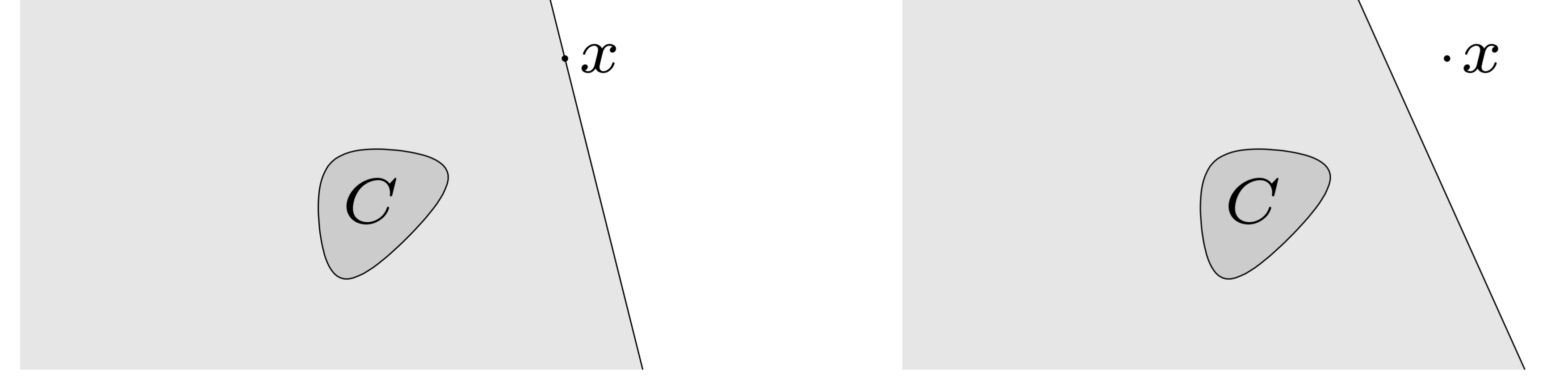
Firgure 1 Left: a neutral cut. Right: a deep cut

When solving the feasibility problem, we proceed as follows: for an initial point $x$, if $x$ satisfies $f_i(x) \leq 0, \forall i$, we return $x$ as a feasible solution. Otherwise, there is at least one constraint that $x$ violates. Let $j$ be the index of one violated constraint where $f_j(x) > 0$; $g_j \in \partial f_j(x)$ be the subgradient value at $x$, from the property of subgradient $f_j(z) \geq f_j(x) + g^T(z-x)$.

we know that once $f_j(x) + g^T (z-x) >0$, then $f_j(z) > 0$, and so $z$ is not a solution. Therefore, for any feasible $z$, it should satisfy $f_j(x) + g^T(z-x) \leq 0$.

In other words, we can remove search space given by the halfspace $f_j(x) + g_j(x)^T(z-x) > 0$. For multiple violated constraints, we can reduce search space by multiple hyperplanes.

To summarize the process of cutting-plane methods, the algorithm goes as

1. given an initial polyhedron $P_0$ that contains $X$, $k:=0$
2. Choose a point $x^{(k+1)} \in P_k$
3. Query the oracle at $x^{(k+1)}$, if the oracle tells $x^{(k+1)} \in X$, return $x$
4. Else, update $P_k$ by cutting-plane: $P_{k+1} := P_k \cap \{z \vert a^T_{k+1}z \leq b_{k+1}\}$
5. Repeat until we find a feasible $x$ or $P_{k+1}$ is empty

Especially, as for a $1-D$ feasible problem, binary search can be regarded as a special cutting-plane method.

From these descriptions, we can know a good cutting-plane method should cut search space in each iteration as big as possible. In other words, the method should minimize the ratio $\frac{Vol(P_{k+1})}{Vol(P_k)}$. According to the strategy of choosing next query point, we have different cutting-plane methods.

Center of Gravity Method

A simple strategy for choosing query point is using the center of gravity. This method was one of the first cutting-plane method proposed by Levin(levin1965algorithm). In this method, we select the center of gravity as the query point $x_{k+1} = cg(P_k)$, where the center of gravity $cg$ is $cg(C) = \frac{\int_C z dz}{\int_C dz}$

Theorem(Grunbaum's inequality) : Given a convex body $K \subseteq R^d$, $x_c := \int _{K}xdx / \int _{K}1dx$, let $H$ be any halfspace that goes through $x_c$ and divide $K$ into $K_1$ and $K_2$, then $\frac{vol(K_1)}{vol(K)} \geq \frac{1}{e}$.

Proof : First, let $K$ be a n-dimensional circular cone, $L=K \cap \{x_1 \leq \overline{x}_1\}$ be the left side of the cone ($x_1$ is the axis of the cone aligned vertex which is at the origin). According to the property of centroid of cone,

$$\frac{vol(L)}{vol(K)} = \frac{vol(\frac{n}{n+1}K)}{vol(C)} = (\frac{n}{n+1})^n$$

Since $\frac{1}{e} \leq (\frac{n}{n+1})^n \leq \frac{1}{2}$, then $\frac{1}{e} \leq \frac{vol(L)}{vol(K)} \leq \frac{1}{2}$

As for any convex body, Without loss of generality, by affine transformation, the centroid can be changed to origin and the hyperplane $H$ used to cut it is $x_1=0$. Then replace every $(n-1)$-dimensional slice $K_t$ with an $(n-1)$-dimensional ball with the same volume to get a convex body $K'$, using Brunn-Minkowski inequality, we can verify that $K'$ is convex. This will not change the ratio of volume that contained in the halfspace. Therefore, we can construct a new cone according to $K'$: let $K'_+ = K' \cap \{x:x_1 \geq 0\}$, $K'_- = K' \cap \{x:x_1 < 0\}$, we replace $K'_+$ with a cone $C$ with the same volume. Similarly, we replace $K'_-$ with an extension $E$ of the cone $C$ with the same volume. After transformation, the centroid of $K'$ is changed from origin to be a little right along $x_1$, note the new centroid as $c^*$.

$$\frac{vol(K_+)}{vol(K)} = \frac{vol(K'_+)}{vol(K')} = \frac{vol(C_+)}{vol(C)} \geq \frac{vol(C_{x_1 \geq c^*})}{vol(C)}$$

From previous result, we know that $\frac{vol(C_{x_1 \geq c^*})}{vol(C)} \geq \frac{1}{e}$, therefore, $\frac{vol(K_+)}{vol(K)} \geq \frac{1}{e}$.

Lemma : By applying Grunbaum’s inequality, the orable complexity of $cg$ is $O(n)$, which means the number of iterations is linear.

Proof : According to Theorem(Grunbaum), we have

$vol(P_k) \leq (1-1/e)^k vol(P_0)$, for a given error tolerance $\epsilon$, assume $f(x) \in [-R, R]$

$$vol(P_k) \leq (1-1/e)^k vol(P_0) \leq (\epsilon/R)^n vol(P_0)$$

Therefore, $k = O(nlog\frac{R}{\epsilon})$

Although the center of gravity method only needs to call oracle within linear times, which achieves the optimal oracle complexity, we need to keep exactly the intersection of all separating hyperplanes and keep record of the feasible region. In addition, this method has a vital disadvantage: the center of gravity is extremely difficult to calculate, especially for a polyhedron in high dimensions. Computing the center of gravity may be more difficult than the optimization problem, which means it is not a practical method.

Analytic Center Cutting-Plane Method

As a variant method of the center of gravity method, the analytic center cutting-plane method(ACCPM)(boyd2008analytic) uses the analytic center of polyhedron as query point. In order to find the analytic center, we need to solve

$$x_{ac} = argmin_z - \sum^m_{i=1}log(b_i-a_i^Tz)$$

where $x_{ac}$ is the analytic center of a set of inequalities $Ax \leq b$. The problem is that we are not given a start point in the domain. One method is to use a phase I optimization method described in (boyd2004convex)(Chapter 11.4) to find a point in the domain and perform standard Newton method to compute the analytic center. Another method is to use an infeasible start Newton method described in (boyd2004convex)(Chapter 10.3), to solve the $argmin$ problem. In addition, we can use standard Newton method to the dual problem.

The dual analytic centering problem is

$$maximize ~ g(z) = \sum^m_{i=1} log z_i - b^Tz$$ $$subject ~ to ~ ~ A^Tz=0$$

The optimality conditions($x,z$ are optimal for primal and dual) are

$$b_i-a_i^Tx=1/z_i, ~ A^Tz=0, ~ z>0, ~ Ax<b$$

Dual feasibility needs

$$A^Tz=z_1-z_2+B^Tz_3=0, ~ z=(z_1,z_2,z_3) \geq 0$$

The Newton equation is

$$\left[ \begin{matrix} -diag(z)^{-2}& A\\ A^{T}& 0\end{matrix} \right] \left[ \begin{matrix} \Delta z\\ w\end{matrix} \right] =\left[ \begin{matrix} b-diag(z)^{-1}1\\ 0\end{matrix} \right]$$

We can solve $(A^Tdiag(z)^2A)w = A^T(diag(z)^2b-z)$ and let $\Delta z=z-diag(z)^2(b-Aw)$.

In order to judge when to finish Newton method, we need Newton decrement

$$\lambda (z) = (\Delta z^T \nabla g(z))^{1/2} = \lVert diag(z)^{-1} \Delta Z \rVert_2$$

When $\lambda(z) =0$, we know $w$ is the analytic center, where $b-Aw=diag(z)^{-1}1$

When $\lambda(z) <1$, we know $x=w$ is primal feasible, where $b-Aw=diag(z)^{-1}(1-diag(z)^{-1} \nabla z) > 0$

The proof for convergence and the analysis of time complexity are a little complex, here we omit the process and take the proof result from Y. Ye(ye2011interior). This algorithm will terminate after $O(\frac{m^2}{\epsilon^2})$ of iterations. The number to call oracle is still linear.

This method was further studied and developed by Vaidya(atkinson1995cutting), which is introduced later.

Ellipsoid Method

Ellipsoid method was developed by Shor, Nemirovsky, Yudin in 1970s and used by Khachian to show the polynomial solvability of Linear Programming problems. Ellipsoid method generates a sequence of ellipsoids with a decreasing volume in $R^n$ that are guaranteed to contain sets of the optimal points. Assume there is an ellipsoid $\varepsilon _{t}$ that is guaranteed to contain a minimizer of $f$. In ellipsoid method, we compute the subgradient $g_t$ of $f$ at the center of ellipsoid, from the result of querying oracle, we then know the half ellipsoid

$$\varepsilon_t \cap \{z \Vert g_{t}^T(z-x_t) \leq 0\}$$

contains the solution. We construct a new ellipsoid $\varepsilon^{k+1}$ with minimum volume that contains the sliced half ellipsoid. We repeat these step until the ellipsoid is small enough to contain a ball with radius $\epsilon$.

Initially, we set $R$ as a large enough number such that $x \subseteq \{x \vert (x-c_1)^TH_1^{-1}(x-c_1)\}$, where $H_1 = R^2I, c_1=\overrightarrow{0}$.

To be exact, we can write the updating of ellipsoid method as a closed form. An ellipsoid $\epsilon$ can be written as $\epsilon = \{z \vert (z-x)^TH_1^{-1}(z-x)\}$, where $H \in S_{++}^n$ which describes the size and shape of ellipsoid, the center of ellipsoid is $x$. The volume of $\epsilon$ is given by $vol(\epsilon) = \beta_n\sqrt{\det H}$, where $\beta_n=\pi^{n/2}/\Gamma(n/2+1)$ is the volume of the unit ball in $R^n$.

The half ellipsoid is

$$\{z \vert (z-x)^TH_1^{-1}(z-x) \leq 1, ~ g^T(z-x) \leq 0\}$$

The new ellipsoid with minimum volume that contains the half ellipsoid is

$$\varepsilon^+=\{z \vert (z-x^+)^T(H^+)^{-1}(z-x^+) \leq 1\}$$

where

$$x^+=x-\frac{1}{n+1}Hg'$$ $$H^+=\frac{n^2}{n^2-1}(H-\frac{2}{n+1}Hg'g'^TH)$$ $$g'=\frac{1}{\sqrt{g^THg}}g$$

According to these formulas, we can calculate the center and shape of ellipsoid in each iteration.

From the notes in this course, we know these theorems.

Theorem : $vol(\varepsilon_{t+1}) \leq exp(-\frac{1}{2n})vol(\varepsilon_t)$

Lemma : The volume of ellipsoid decreases by a constant factor after $n$ iterations. The iteration number is $O(n^2log\frac{1}{\epsilon})$

From the calculation process, ellipsoid method takes $O(n^2log\frac{1}{\epsilon})$ calls of oracle, which is far from the lower bound $O(nlog\frac{R}{\epsilon})$. We find that the separating hyperplane is only used for producing the next ellipsoid. In fact, ellipsoid method is theoretically slower than interior point method and practically very slow since it always does the same computation. However, ellipsoid method is still a quite important theory, as the black-box property enables us to solve exponential size linear programming problem.

The Volumetric Center Method by Vaidya

By maintaining an approximation of the polytope and using a different center, which is called volumetric center, Vaidya(atkinson1995cutting) obtained a faster cutting-plane method.

The idea comes from interior point method that to compute an approximation of the volumetric center. The approximation is obtained by using the previous center as the initial solution to compute the center of the current center by Newton method.

Let $C$ be the convex set which is approximated by a finite set of inequalities, so $C\subseteq \{x:A^Tx \leq c\}=: Q$ ($A$ is an $m \times n$ matrix and $c$ is an $n$-vector).Let $x$ be a strictly feasible point in $Q$ and $s = c-A^Tx > 0$. The logarithmic barrier $F$ for the polytope is

$$F(x)=-\sum_{i=1}^m \log(a_i^Tx-b_i)$$

Therefore, based on the logarithmic barrier, we can obtain the volumetric barrier function for $Q$ at point $x$:

$V(x):=\frac{1}{2}\log\det(\nabla ^{2}F\left( x\right))​$, where $\nabla ^{2}F\left( x\right) = \sum_{t=1}^m \frac{a_ia_i^T}{(a_i^Tx-b_i)^2}​$

By setting the $V(x)$ in this form, in fact, $V(x)$ is the inverse volume of the Dikin ellipsoid at point $x$. Volumetric barrier can be regarded as a weighted log-barrier. By introducing the leverage scores of constraints

$$\sigma_i(x)=\frac{a_t^T(\nabla ^{2}F\left( x\right))^{-1}a_i}{(a_ix-b_i)^2}$$

we can verify $\nabla V(x) = -\sum_{i=1}^m \sigma_i(x) \frac{a_i}{a_i^Tx-b_i}$

In fact, Vaidya’s method produces a sequence of pairs $(A_t, b_t) \in R^{mn} \times R^m$ such that the corresponding polytope contains the convex set of interest. The initial polytope is a simplex or a hypercude that is guaranteed to contain the convex set. In each iteration, we compute the minimizer of the volumetric barrier of the polytope given by $(A_t, b_t)$ and the leverage score at the point $x_t$. The next polytope $(A_{t+1}, b_{t+1})$ is generated by either adding or removing a constraint from current polytope.

Therefore, with these notations, Vaidya’s method can be described as:

1. set a small value $\epsilon \leq 0.006$
2. in each iteration, compute the volumetric center by taking $x_{t-1}$ as the initial point for Newton’s method
3. if $\exists i, \sigma_i = \min \sigma_j < \epsilon$, simply remove the $i$-th constraint
4. otherwise let c be the vector given by the separation oracle, by choosing $\beta$ that satisfies $\frac{c^T \nabla ^{2}F\left( x\right)^{-1}c}{(x^Tc-\beta)} = \frac{1}{5}\sqrt{\epsilon}$ we add the constraint $c^Tx \geq \beta$ given by $(c, \beta)$ to the polytope.
5. return the best center during iterations.

The idea is straightforward: by introducing the leverage score which reflects the importance of each constraint, we can drop an unimportant constraint during iteration and the volume decreases with a value proportional to the leverage score; Otherwise this constraint is important, then we add it to the polytope.

Lemma : In Step.3, by removing the $i$-th constraint, the volume of the Dikin ellipsoid does not change dramatically as

$$V_{t+1}(x_{t+1}) - V_t(x_t) \geq -\epsilon$$

Lemma : In Step.4, by adding the $i$-th constraint, the volume of the Dikin ellipsoid does not change dramatically as

$$V_{t+1}(x_{t+1}) - V_t(x_t) \geq \frac{1}{20}\sqrt{\epsilon}$$

Lemma : Vaidya’s method stops after $O(n \log (nR/r))$ steps. The computational complexity is $O(n^4)$

Vaidya’s method uses Newton’s method to compute the volumetric center, which could be very fast. The computational bottleneck comes from computing the gradient of $\log\det$, where we need to compute the leverage score $\sigma_i(x)$. So far, the best algorithm for computing leverages scores can improve the computational complexity from $O(n^3)$ to $O(n^w), w\approx2.37$.

A Faster Cutting Plane Method by Lee, Sidford and Wong

This recent method by Lee, Sidford and Wong(lee2015faster) is built on top of Vaidya’s method focusing on the improvement on leverage scores. Although, instead of computing the exact leverage score, we can make an approximation with $(1\pm\epsilon)$ error and achieve $O(\epsilon^{-2}\log n)$ time complexity, Vaidya’s method does not tolerate the multiplicative error. As a result, the approximated center is not close enough to the actual volumetric center, leading to a insufficient query to separation oracle.

Previously in Vaidya’s method, the volumetric center is defined as

$$V(x):=\frac{1}{2}\log\det(\nabla ^{2}F\left( x\right))$$

where $\nabla ^{2}F\left( x\right) = \sum_{t=1}^m \frac{a_ia_i^T}{(a_i^Tx-b_i)^2}$

Now for convenience, we note $S=Ax-b, s_i \in S$, then

$$\nabla ^{2}F\left( x\right)= A^TS^{-2}A, ~ ~ ~ ~ V(x):=\frac{1}{2}\log\det(\nabla ^{2}F\left( x\right)) = \frac{1}{2}\log\det(A^TS^{-2}A)$$

Based on these fact, the authors came up with a hybrid barrier function as:

$$\arg\min_x -\sum_i w_i \log s_i(x) + \log \det (A^TS^{-2}A)$$

where $w_i$ is the weight which is chosen carefully so that the gradient of this function can be computed. For example, let $w = \tau - \sigma(x)$, we reduce the problem as taking the gradient of $\sum_i \tau_i \log s_i(x)$. The authors also observe that the leverage score does not change greatly between iterations, then they suggests an unbiased estimates to the change of leverage score can be used such that the total error of the estimate is bounded by the total change of the leverage scores. In addition, instead of minimizing the hybrid barrier function, the authors set the weights so that Newton’s method can be applied, as the accurate unbiased estimates of the changes of leverage score is computed, the weights will not change dramatically.

To conclude, this hybrid barrier function takes these assumptions:

• The weights will not change too much between iterations. By carefully choosing the index, no weight will get too large.

• The changing on weights makes a bounded influence on $\log \det$. To make sure this, the authors add a regularization term. The modified function is $p(x)=-\sum_i w_i \log s_i(x) + \frac{1}{2}\log\det(A^TS^{-2}A) + \frac{\lambda}{2} \lVert x \rVert_2^2$

• The hybrid barrier function is convex, this is guaranteed by setting $w=c_e+\tau-\sigma$ such that $\lVert \tau-\sigma \rVert_{\infty} < c_e$.

Therefore, the algorithm can be described as

1. Start from a Ball that contains $K$, where $K$ stands for the feasible set. Set $\epsilon$ as threshold.
2. In each iteration $T$, we find $w_i$ such that
   • $\frac{1}{2}\sigma_i(x^{(T)}) \leq w_i^{(T)} \leq 2\sigma_i(x^{(T)})$.
   • $\lVert w_i^{(T+1)} - w_i^{(T)} \rVert$ is small, say $\lVert w_i^{(T+1)} - w_i^{(T)} \rVert \leq 0.001$
   • $Ew_i^{(T+1)} = w_i^{(T)} + \sigma_i^{(T+1)} - \sigma_i^{(T)}$.
3. Therefore, we store previous $w_i$, update $w_i$ using dimension reduction.
4. Check the error of estimation, if estimation is too bad, we compute it exactly(Set $w_i=0$).
5. Similarly as Vaidya’s method, we use these approximated leverage scores to remove constraints or add constraints.
6. return a feasible point $x$ or conclude that there is no such point.

In particular, the hybrid barrier function becomes

$$p_e(x) := -\sum_i(c_e + e_i) \log s_i(x) + \frac{1}{2}\log \det (A^TS^{-2}A+\lambda I) + \frac{\lambda}{2}\lVert x \rVert_2^2$$

where $e\in R^m$ is the variable we maintain. The reason why there is $\lambda I$ in the $\log \det$ term is that the $l_2$ norm changes the Hessian of origin function, this term is added to reflect the change. Instead of maintaining $e$ directly, the authors maintain a vector $\tau \in R^m$ that approximation the leverage score

$$\psi(x) := diag (A(A^TA+\lambda I)^{-1}A^T)$$

Lemma(Time complexity) : Let $K \subseteq R^n$ be a non-empty set in a ball with radius $R$. For any $\epsilon \in (0, R)$, within expected time $O(n \log(nR/\epsilon) + n^3 \log^{O(1)}(nR/\epsilon))$, this method can output a point $x\in K$ or conclude there is no feasible point.

The clever idea in this method is that the authors keep a track on the change of $w_i$, by setting $w_i$ correctly, they transform computing leverage score into a linear system problem. Therefore, compared to Vaidya’s method, where the leverage score is computed exactly, this method uses bounded approximation of leverage score, the time complexity in computing leverage score is reduced from $O(n^w)$, where $w\approx 2.37$ to $O(n^2)$. Follow the same analysis process in Vaidya’s method, we can conclude that the general time complexity is $O(n \log(nR/\epsilon) + n^3 \log^{O(1)}(nR/\epsilon))$.

In fact, all the theorems and assumptions are proved in the origin paper, as the proofs are complex and complete, please refer to the paper(lee2015faster) for more details.

A New Polynomial Algorithm by Chubanov

This method is a very recent result, the interesting part is the method does not need the notion of volume to prove the polynomial complexity.

The idea in this paper is based on rescaling(or space dilation) in ellipsoid method, but the final algorithm is a non-ellipsoidal algorithm that solves linear systems in polynomial oracle time.

Theorem(Caratheodory's Theorem) : Let $A \in R^d$, $C=ConvA$ as its convex hull, then

$$C=\{\sum_{i=1}^t \lambda_ia_i : \lambda_i \geq 0, \sum_{i=1}^t \lambda_i =1, a_i \in A, t=1,2,...,d+1\}$$

Proof : Carath'eodory’s theorem shows at most d+1 points are needed to describe C.

Suppose x in a point in C and $x=\sum_{i=1}^{t} \lambda_i a_i:\lambda \geq 0, \sum_{i=1}^{t} \lambda_i=1, t \geq d+2$, x is the convex combination of at least d+2 points. for $a_1, a_2,...,a_k \in A$, consider they are affinely independent. Then there exists $\mu_1, \mu_2, ... , \mu_t$, not all zero, such that $\sum_{i=1}^{t} \mu_i a_i =0 \ and \ \sum_{i=1}^{t} \mu_i = 0$.

$$x = \sum_{i=1}^{t} \lambda_i a_i - \theta \times 0 = \sum_{i=1}^{t} \lambda_i a_i - \theta \sum_{i=1}^{t} \mu_i a_i = \sum_{i=1}^{t} (\lambda_i - \theta \mu_i)a_i : \theta \in R$$

Since $\sum_{i=1}^{t} \mu_i = 0$ and not all $\mu_i$ are zero, there are positive $\mu_i$ and negative $\mu_i$. Let $\theta = min\frac{\lambda_a}{\mu_a}$, $\mu_a$ is in positive $\mu_i$, one of the coefficients in $\lambda_i - \theta \mu_i$ is 0 and $\forall i, \lambda_i - \theta \mu_i \geq 0$. What’s more, $\sum_{i=1}^{t} \lambda_i-\theta \mu_i = \sum_{i=1}^{t} \lambda_i - \theta \sum_{i=1}^{t} \mu_i = 1$, here point x can be represented as combination of points without point $a_a$. Then t could be reduced by 1. This process could be repeated as long as there are affinely independent points in the t points.

The maximum number of affinely independent points in $\mathbb{R}^d$ is d+1, in other words, t could be only reduced to $d+1$.

Lemma : for a matrix $A$, any convex combination of the rows of A can be represented in the form $A^Ty$ where $y$ has no more than $n+1$ nonzero components, and $y$ satisfies $y\geq0, ~ \sum_i y_i=1, \lVert y \rVert_{\infty} \leq n+1 \leq 2n$

Let $y_k$ be the maximum entry of $y$, from previous lemma, we know $\frac{1}{2n} \leq y_k \leq 1$. Let $A_k$ be the related row in $A$. For a vector $a$, let $\Delta = A_k^T - a$, for any $x$ satisfies $Ax \geq 0$, we know

$$\frac{1}{2n} \vert a^Tx \vert \leq y_k \vert a^Tx \vert = \vert y_k(A^T_k - \Delta)^Tx) \vert \leq (\lVert y^T A \rVert + \lVert \Delta \rVert) \lVert x \rVert$$

Lemma(oracle complexity) : Given $\epsilon \in [0,1]$, within $O(\frac{n^2}{\epsilon^2})$ oracle calls and $O(\frac{n^4}{\epsilon^2})$ arithmetic computations, we can find a solution of feasible problem or a vector $a$ such that

$$\lVert a \rVert^2 \in [1,2], ~ \vert a^T x \vert \leq \epsilon \lVert x \rVert$$

Proof : During the iterations, when we check a nonzero vector, assume the $l$-th is violated(otherwise we are done). Let $y=e_l$ be the vector that only the $l$-th entry is 1 and 0s in other entries, we check whether $A^Ty \leq 0$. If so, we return $y$ as the solution, otherwise, let the new violated constraint as $i$-th entry of A, i.e. $A_ix \geq 0$. Let $y' = \alpha y + (1-\alpha)e_i$, where

$$\alpha = \frac{A_i (A_i^T - A^Ty)}{\lVert A_i^T - A^Ty \rVert ^2}$$

From geometrical perspective, when the origin is orthogonally projected to $[A^Ty, A^T_i]$, we obtain $A^Ty'$. If $\lVert A^Ty'\rVert = 0$, we find a feasible solution. Otherwise, according to rescaling of $A$, we can bound $\lVert A_i \rVert^2 \in [1, \frac{3}{2}]$, we know

$\frac{1}{\lVert A^Ty' \rVert^2} \geq \frac{1}{\lVert A^Ty \rVert^2} + \frac{1}{\lVert A_i \rVert^2} \geq \frac{1}{\lVert A^Ty \rVert^2} + \frac{1}{2}$, where $\lVert y' \rVert_{\infty} - \lVert y \rVert_{\infty} \leq 1$.

Then we set $y=y'$ and repeat these steps. From this inequality, we know that the decreasing rate of $y$, the number of iterations is bounded by $O(\frac{n^2}{\epsilon^2})$. In order to compute $y'$ at each iterations, we need to call the separation oracle and check every constraint, which results in $O(n)$ arithmetic operations in each iteration. Since $\lVert y' \rVert_{\infty} - \lVert y \rVert_{\infty} \leq 1$, the number of nonzero entries in $y$ increases at most 1 between iterations. Then a $O(n^3)$ algorithm is used after $n$ iterations, where $O(n^3)$ comes from the algorithm that solves $A^T_Jv = A^Ty', \sum_i v_i = 1, v_i \geq 0$. By taking all conditions, we obtain the wanted complexity analysis.

Consider two orthogonal vectors $a\in R^n, w \in R^n, a^Tw=0$, we know that for any $x \in R^n$, x is uniquely represented by $w, a$. Therefore, any function for $x$ and be regard as function for $(w, a)$. Let $f$ be the linear operator as $f(x) = f(w, a) = w + 2\lambda a$

Lemma : Let $1 \leq \lVert a \rVert^2 \leq 2$, set $x$ such that $\Vert a^Tx \Vert \leq \frac{\lVert x \rVert}{\sqrt{6n}}$, then $\lVert f(x) \rVert \leq \lVert x \rVert \sqrt{\frac{n+1}{n}}$

Proof : As $x$ can be represented as $x = w+\lambda a$, from $\Vert a^Tx \Vert \leq \frac{\lVert x \rVert}{\sqrt{6n}}$, $\Vert \lambda \Vert \lVert a \rVert^2 = \Vert a^Tx \Vert$, $\lVert a \rVert^2 \geq 1$, we know $\Vert \lambda \Vert \leq\frac{\lVert x \rVert}{\sqrt{6n}}$. Therefore,

$$\lVert f(x) \rVert^2 = \lVert w+2\lambda a \rVert^2 = \lVert w \rVert^2 + 4\lambda^2 \lVert a \rVert^2 = \lVert x \rVert^2 + 3\lambda^2 \lVert a \rVert^2 \leq \lVert x \rVert^2 + \frac{\lVert x \rVert^2}{n}$$

Then $\lVert f(x) \rVert \leq \lVert x \rVert \sqrt{\frac{n+1}{n}}$.

Consider the feasible constraints as $Ax \geq 0$. As the beginning of this method, it assumes the $l_2$ norms of the rows in $A$ is bounded in $[1, \frac{3}{2}]$, if they are not in the range, simply normalize the coefficient vector.

The algorithm is described as

1. Let $D$ begin as the identity matrix.
2. Let $A'$ be the matrix obtained from normalizing the rows such that $\lVert a'_i \rVert \in [1, \frac{3}{2}]$. Given a vector $v$, use a polynomial procedure to find a value $\gamma$ such that $\gamma^2 \lVert v \rVert^2 \in [1, \frac{3}{2}]$. Then, $A'=\gamma A_iD$. Set $\epsilon = \frac{1}{\sqrt[]{6n}}$, find a nonzero vector $z$ such that $z=A'^Ty$ satisfies $A'x \geq 0$ or a vector $a$ such that $\lVert a \rVert^2 \in [1,2], \Vert a^Tx \Vert \leq \frac{\lVert x \rVert}{\sqrt[]{6n}}$ for all $x$ with $A'x \geq 0$.
3. if $z$ is found, return $x^*= Dz$
4. Otherwise, set $D=D(I-\frac{1}{2\lVert a \rVert^2}aa^T)$
5. repeat steps until, the number of iterations exceed limit.

From above setting, $x$ is feasible for $Ax \leq 0$ if and only if $x$ satisfies this system(Let $A_ix \geq 0$ be violated at $x'=Dx$, then $\gamma A_iDx \geq 0$ is violated at $x'$). We use the separation oracle for $Dx$ and compute $\gamma$, where $\gamma$ is computed from violated constraints and normalization procedure.

In the iteration, by setting $\epsilon$, we make sure $\Vert a^Tx \Vert \leq \frac{\lVert x \rVert}{\sqrt[]{6n}}$. from the result in Lemma, for each column in $X$,

$$\lVert D^{-1} x \rVert = \lVert f(x) \rVert \leq \lVert x \rVert \cdot \sqrt[]{1+\frac{1}{n}} \leq \sqrt[]{1+ \frac{1}{n}}$$

Theorem(Sylvester's determinant identity) : Given $A\in R^{m \times n}, B\in R^{n \times m}$, the equation holds

$$\det(I_m + AB) = \det(I_n + BA)$$

Proof : Construct $M$ as

$$M=\left[ \begin{matrix} Im& -A\\ B& In\end{matrix} \right]$$

as $I_m$ has its inverse $I_m^{-1}$,

$$\det(M) = \det(I_m) \det(I_n - B I_m^{-1} (-A)) = \det(I_n + BA)$$

as $I_n$ has its inverse $I_n^{-1}$,

$$\det(M) = \det(I_n) \det(I_m - (-A) I_n^{-1} B) = \det(I_m + AB)$$

Therefore, $\det(I_m + AB) = \det(I_n + BA)$

Theorem(Hadamard's inequality) : Let $a_i$ be column in $A$, then $\Vert \det(A) \Vert \leq \prod_i \lVert a_i \rVert$

Proof : It is obvious that if $\det(A) = 0$, the inequality holds as $l_2$ norm is non-negative. When $\det(A) \neq 0$, this suggests that all columns in $A$ are linear independent. Therefore, we can orthogonalize these columns. Let $E_j = span(a_1, ... , a_j)$, $P_j$ be the orthogonal project onto $E_j$, $b_1=a_1$ and $b_j=P_{j-1}(a_j)$, then $\lVert b_j \rVert \leq \lVert a_j \rVert, \forall j \in [2, n]$. Also, we have

$$b_j = a_j - \sum_{i=1}^{j-1} \frac { < a_{j},b_{i}>} { < b_{i}\cdot bi>}b_{i}, \forall j \in [2, n]$$

Let $B$ be the matrix with columns $b_i$, $B$ is obtained from $A$ by elementary column operations, then $\det B=\det A$. Since the columns in $B$ are orthogonal, we have $B^TB = diag(\lVert b_1 \rVert^2, \lVert b_2 \rVert^2, ... , \lVert b_n \rVert^2)$. Therefore,

$$\Vert \det A \Vert = \Vert \det B \Vert = (\det(B^TB)^{1/2} = \prod_{j=1}^n \lVert b_j \rVert) \leq \prod_{j=1}^n \lVert a_j \rVert$$

According to Sylvester’s determinant identity, $det(I+\frac{1}{\lVert a \rVert^2}aa^T)=1+\frac{\lVert a \rVert^2}{\lVert a \rVert^2} = 2$, therefore, according to Hadamard’s inequality, $2 \Vert \det x \Vert = \Vert \det D_{-1}X \Vert \leq (\sqrt[]{1+\frac{1}{n}})^n < e^{1/2}$

After $T$ iterations, from previous analysis, we obtain

$$2^T \Vert \det X \Vert = \Vert \det D^{-1} X \Vert \leq (\sqrt[]{1+\frac{1}{n}})^{nT} \leq e^{T/2}$$

Lemma : Let $X^*$ be a feasible matrix with the maximum determinant during iterations, this algorithm can return a solution in $O(n^3\log( \Vert \det X^* \Vert ^{-1}))$ calls in separation oracle and $O((n^5+n^3T)\log( \Vert \det X^* \Vert ^{-1}))$ arithmetic operations.

Although the total time complexity is quite weak compared to previous cutting-plane method, the Chubanov’s method gives us an interesting perspective of the usage of separation oracle.

Conclusion

Most people may believe that cutting-plane method is only meaningful for theoretic analysis and unpractical for real applications. It is a common sense that compared to computing gradient or Hessian, maintaining the volume and center of ellipsoid is relatively slow. However, according to a recent paper by Bubeck, Lee, and Singh(bubeck2015geometric), cutting-plane method is suitable for real applications. For short, we name steepest decent as “SD”, accelerated full gradient method as “AFG”, accelerated full gradient method with adaptive restart as “AFGwR”. All of them are first-order optimization algorithms. In addition, we note quasi-Newton with limited-memory BFGS updating as “L-BFGS”, note geometric decent as “GeoD” which is exactly the cutting-plane method.

We know Newton’ method is the optimal bound for optimization problem and gradient decent with its variants are prevailing algorithms. The authors tested the performance of all algorithms on 40 datasets and 5 regularization coefficients with smoothed hinge loss function. The results are as follows:

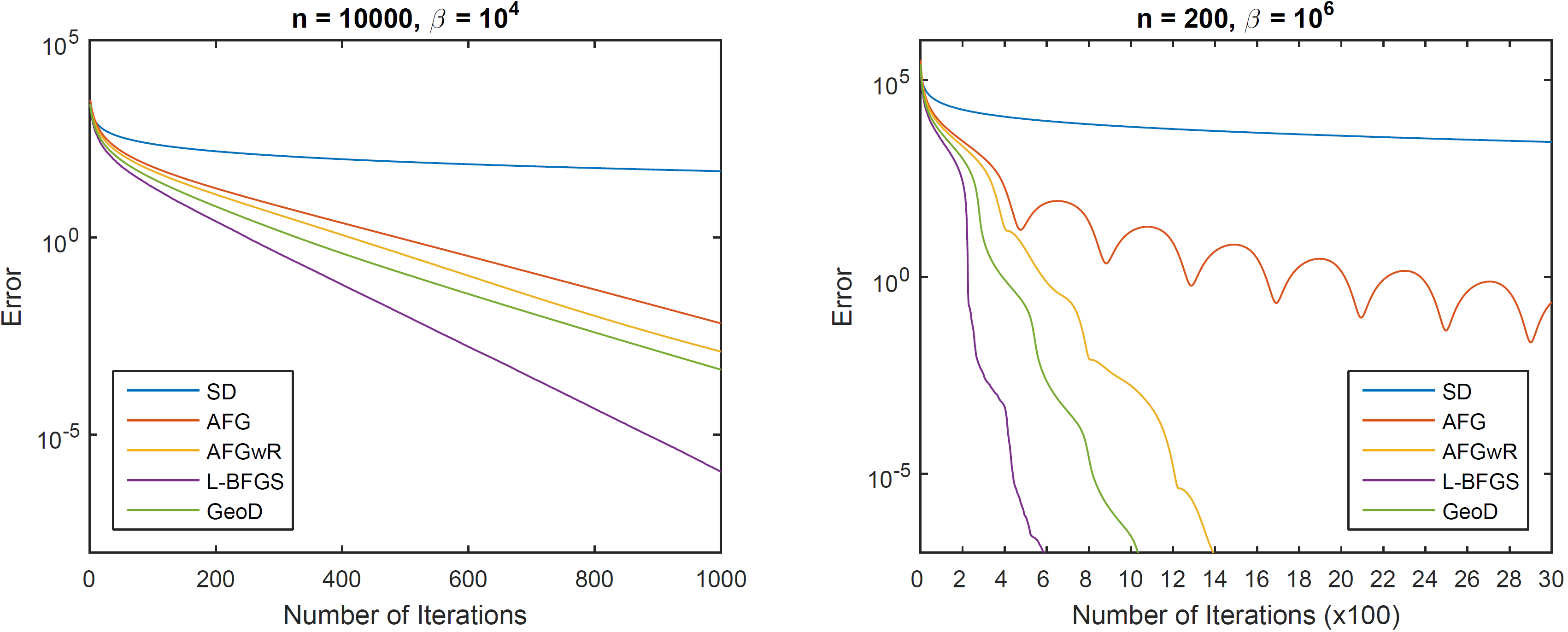
Comparison of gradient methods and cutting-plane method

From this figure, we find that cutting-plane is surprisingly suitable for optimization problem in real application. As Hessian matrix in Newton’s method is extremely difficult to maintain; gradient descent should set up with a careful step size, cutting-plane methods has the advantages in converging speed and computing complexity. We may see more developments and applications of cutting-plane methods in the future.

Acknowledge

Thank Professor Lap Chi Lau for feedbacks and suggestions. Also, thank Professor Yaoliang Yu for inspiring and providing some helps during this blog.

Ruifan Yu

Welcome! My name is Ruifan Yu. I am currenly a Software Engineer in Google, exploring the fabulous ocean of Computer Science.